Introduction to Polars
Polars is a Python library written in Rust to manipulate data. As it has been gaining traction over the last few years, I will discuss here what are its main advantages and how to get started
Sources
- Official Guide: https://docs.pola.rs/user-guide/getting-started/
- Real python introduction: https://realpython.com/polars-python/
- Pandas vs Polars: https://blog.jetbrains.com/pycharm/2024/07/polars-vs-pandas/
- Benchmarks: Database-like ops benchmark
Why Polars?
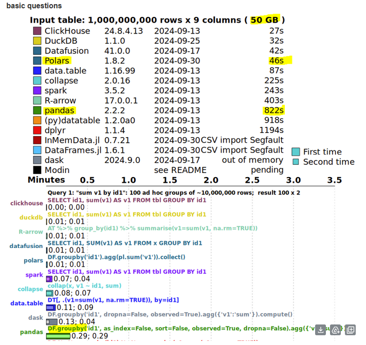
Because it is fast: “Polars is between 10 and 100 times as fast as pandas for common operations […]. Moreover, it can handle larger datasets than pandas can before running into out-of-memory errors”.
Benchmark example: see more at https://duckdblabs.github.io/db-benchmark/
It has a few interesting features:
- “Pandas, by default, uses eager execution, carrying out operations in the order you’ve written them. In contrast, Polars has the ability to do both eager and lazy execution, where a query optimizer will evaluate all of the required operations and map out the most efficient way of executing the code”
- Similar to SQL, you can get a “lazy (SQL) plan graph”, showing you the various steps that Polars will take to execute your operation
- Polars can “scan” a dataset, meaning you don’t have to load an entire static file before processing it. Therefore: “it allows you to process large datasets stored in files without reading all the data into memory.”
- A lot of functions have the same names as their pandas’s equivalent, so the learning process can be smoother
To get started
As you can see below, all the classic functions head(), tail(), Dataframe(), describe() are similar to Pandas.
You can also use things like: df.write_csv(“docs/assets/data/output.csv”) or convert pandas dataframe with from_pandas() & to_pandas()
Input
import polars as pl
import datetime as dt

df = pl.DataFrame(
{
"name": ["Alice Archer", "Ben Brown", "Chloe Cooper", "Daniel Donovan"],
"birthdate": [
dt.date(1997, 1, 10),
dt.date(1985, 2, 15),
dt.date(1983, 3, 22),
dt.date(1981, 4, 30),
],
"weight": [57.9, 72.5, 53.6, 83.1],  # (kg)
"height": [1.56, 1.77, 1.65, 1.75],  # (m)
}
)
print(df)
print(df.head())
print(df.describe()
Concepts Overview: expressions and contexts
Expressions are operations on a column. Contexts is the situation in which your expression is evaluated.
- Expressions can be arithmetic calculations, performing comparisons, etc.
- Contexts can be of 3 types: Selecting, Filtering or Groupby/aggregation
Contexts
“Select” context
result = df.select(
    pl.col("name"),
    pl.col("birthdate").dt.year().alias("birth_year"),
    (pl.col("weight") / (pl.col("height") ** 2)).alias("bmi"),
)

print(result))
In this example, “select” is a context and each expression maps a column of the output dataframe
“with columns” context
"with_columns adds columns to the dataframe instead of selecting them"
result = df.with_columns(
    birth_year=pl.col("birthdate").dt.year(),
    bmi=pl.col("weight") / (pl.col("height") ** 2),
)

print(result)
Input with “Filter” context
result = df.filter(
    pl.col("birthdate").is_between(dt.date(1982, 12, 31), dt.date(1996, 1, 1)),
    pl.col("height") > 1.7,
)

print(result)
“Group by” context
result = df.group_by(
    (pl.col("birthdate").dt.year() // 10 * 10).alias("decade"),
    maintain_order=True,
).len()

print(result)
Another example with aggregations on the top of it
result = df.group_by(
    (pl.col("birthdate").dt.year() // 10 * 10).alias("decade"),
    maintain_order=True,
).agg(
    pl.len().alias("sample_size"),
    pl.col("weight").mean().round(2).alias("avg_weight"),
    pl.col("height").max().alias("tallest"),
)

print(result))
Everything together
result = (
    df.with_columns(
        (pl.col("birthdate").dt.year() // 10 * 10).alias("decade"),
        pl.col("name").str.split(by=" ").list.first(),
    )
    .select(
        pl.all().exclude("birthdate"),
    )
    .group_by(
        pl.col("decade"),
        maintain_order=True,
    )
    .agg(
        pl.col("name"),
        pl.col("weight", "height").mean().round(2).name.prefix("avg_"),
    )
)
print(result)
The Lazy API
The lazy API is Polar’s main strength and allows it to :
- apply automatic query optimization with the query optimizer
- work with larger-than-memory datasets using streaming
- catch schema errors before processing the data
The main idea is that you specify a sequence of operations without immediately running it. “Instead, these operations are saved as a computational graph and only run when necessary”.
LazyFrames
To use the lazy API, we have to start by creating a lazy frame. This can be done in different ways, such as using the LazyFrame() method, as seen below. You can also convert an existing data frame with lazy().
num_rows = 5000
rng = np.random.default_rng(seed=7)

buildings = {
      "sqft": rng.exponential(scale=1000, size=num_rows),
      "price": rng.exponential(scale=100_000, size=num_rows),
      "year": rng.integers(low=1995, high=2023, size=num_rows),
      "building_type": rng.choice(["A", "B", "C"], size=num_rows),
}

buildings_lazy = pl.LazyFrame(buildings)
You can then create a query. The query is not executed
lazy_query = (
    buildings_lazy
    .with_columns(
        (pl.col("price") / pl.col("sqft")).alias("price_per_sqft")
    )
    .filter(pl.col("price_per_sqft") > 100)
    .filter(pl.col("year") < 2010)
 )

lazy_query # not executed
Query plan
You can have a nice visualization if you have Graphviz installed. The visualization is read from bottom to top where:
- each box corresponds to a stage in the query plan
- the
sigmastands forSELECTIONand indicates any filter conditions - the
pistands forPROJECTIONand indicates choosing a subset of columns
lazy_query.show_graph()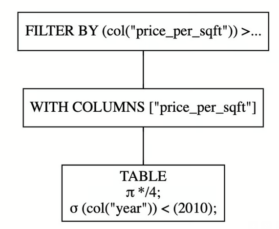
“You can interpret the full query plan with these steps:
- Use the four columns of
buildings_lazy, and filterbuildings_lazyto rows whereyearis less than 2010. - Create the
price_per_sqftcolumn. - Filter
buildings_lazyto all rows whereprice_per_sqftis greater than 100."
Alternatively, we can use explain(), which gives us the following text result. Similarly to the graph, you read it from bottom to top, and each line is a stage.
FILTER [(col("price_per_sqft")) > (100.0)] FROM
   WITH_COLUMNS:
   [[(col("price")) / (col("sqft"))].alias("price_per_sqft")]
    DF ["sqft", "price", "year", "building_type"]; PROJECT */4 COLUMNS; SELECTION: [(col("year")) < (2010)]
Both explain() and show_graph() take for argument optimized=False to see what the non optimized plan looks like
Executing
Executing is done with the collect method
lazy_query = (
    buildings_lazy
    .with_columns(
        (pl.col("price") / pl.col("sqft")).alias("price_per_sqft")
    )
    .filter(pl.col("price_per_sqft") > 100)
    .filter(pl.col("year") < 2010)
 )
(
    lazy_query
    .collect()
    .select(pl.col(["price_per_sqft", "year"]))
)
The Usecase
The main reason to use the Lazy API is to apply operations on a static file like csv without fully loading the file into memory. “When working with files like csv, you’d traditionally read all of the data into memory prior to analyzing it. With Polars’ lazy API, you can minimize the amount of data read into memory by only processing what’s necessary. This allows Polars to optimize both memory usage and computation time
So rather than reading the entire file into memory, instead you scan it to createa LazyFrame that references the file’s data
lazy_car_data = pl.scan_csv(local_file_path)
lazy_car_data

# give lazy_car_data.schema
# {'VIN (1-10)': Utf8, 'County': Utf8, 'City': Utf8, 'State': Utf8,
# 'Postal Code': Int64, 'Model Year': Int64, 'Make': Utf8, 'Model': Utf8,
# ...
“You can now query the data contained in electric_cars.csv using the lazy API. Your queries can have arbitrary complexity, and Polars will only store and process the necessary data"
lazy_car_query = (
    lazy_car_data
    .filter((pl.col("Model Year") >= 2018))
    .filter(
        pl.col("Electric Vehicle Type") == "Battery Electric Vehicle (BEV)"
    )
    .groupby(["State", "Make"])
    .agg(
        pl.mean("Electric Range").alias("Average Electric Range"),
        pl.min("Model Year").alias("Oldest Model Year"),
        pl.count().alias("Number of Cars"),
    )
    .filter(pl.col("Average Electric Range") > 0)
    .filter(pl.col("Number of Cars") > 5)
    .sort(pl.col("Number of Cars"), descending=True)
)

lazy_car_query.collect() # no computation is performed until you call collect